Batter’s ball Striking Zones Analytics (Cricket) and using Dash Plotly to make it into an interactive web app.
With a dash of Data science

Analyzing any opponent’s past performances is a crucial step in preparing for a matchup in any sport. This helps identify the strengths and weaknesses of the opponent, which can help athletes prepare better for the upcoming challenge. Likewise in Cricket, studying the opposition’s batter’s is a crucial part of the process, recognizing the batter’s strength and weakness helps the team to come up with a plan on which areas to bowl to a particular batter. Inspired by the infographics used by the cricket broadcaster, I have prepared the same plot in python using the Plotly library.
Data Preparation
Since such data is not made available by the broadcaster’s, I went ahead and created synthetic data for plotting these graphs. Below is the screenshot of the data created :

The x and y coordinate columns represent the point where the ball was delivered in a 2D space with respect to the image on which these points are superimposed. Events column unique values are ‘white’: Wicket ball(i.e. ball on which the batter got out), ’red’: Dot ball (i.e. ball on which no runs was scored), ’goldenrod’: Boundaries (either a Four or a Six), ‘blue’: Runs scored apart from boundaries (i.e. Singles, Doubles, and triples). I have generated these values with a specific probability distribution using python library random and choices.
events_color = ['white','red','goldenrod', 'blue']
events_probability_distribution = [0.075,.525,0.25,0.15]
The Runs column contains an integer corresponding to the color in the events column. For colors ‘white’ and ’red’ the run scored will be 0, for ‘goldenrod’ it’s either a 4 or 6 and for ‘blue’ one of the three 1,2, and 3 with a predefined probability of all.
# boundaries with probabilty distribution
boundaries = [4, 6]
probability_distribution = [.8, .2]
# 1's 2's 3's with probabilty distribution
runs = [1,2,3]
probability_distribution = [0.5,.35,.15]
The last column is zones which contains 5 unique zone values according the the value in the x coordinate column.
Infographics
Using the above-created data, and the stumps image I downloaded from the internet. Created a scatter plot using Plotly to plot x and y coordinates superimposed over the image. The below code was used to generate the plot :
fig = go.Figure()
# Add image
img_width = 432
img_height = 264
scale_factor = 0.5
fig.add_layout_image(
        x=0,
        sizex=img_width,
        y=0,
        sizey=img_height,
        xref="x",
        yref="y",
        opacity=1.0,
        layer="below",
        source="assets/pitch.PNG"
)
fig.update_xaxes(visible=False,showgrid=False, range=(0, img_width))
fig.update_yaxes(visible=False,showgrid=False,scaleanchor='x', range=(img_height, 0))fig.add_trace(go.Scatter(x=f.x,
                         y=f.y,
                         mode='markers',
                         text=f['Runs'],
                         marker=dict(size=20,color=f.events.to_list())))

Also, we have to create zones corridors and mark them sequentially, for that plotly provides methods such as add_vrect and add_annotation. Below is the code used :
fig.add_vrect(
    x0=202, x1=237,
    fillcolor="LightSalmon", opacity=0.3,
    layer="above", line_width=0,
),
fig.add_vrect(
    x0=237, x1=279,
    fillcolor="turquoise", opacity=0.3,
    layer="above", line_width=0,
),fig.add_vrect(
    x0=167, x1=202,
    fillcolor="LightSeaGreen", opacity=0.3,
    layer="above", line_width=0,
),fig.add_vrect(
    x0=132, x1=167,
    fillcolor="lightgoldenrodyellow", opacity=0.3,
    layer="above", line_width=0,
),fig.add_vrect(
    x0=90, x1=132,
    fillcolor="goldenrod", opacity=0.3,
    layer="above", line_width=0,
),fig.add_annotation(
        x=112,
        y=250,
        xref="x",
        yref="y",
        text="Zone 1",
        showarrow=False,
        font=dict(
            family="Courier New, monospace",
            size=16,
            color="#ffffff"
            ),
        align="center",
        bordercolor="#c7c7c7",
        borderwidth=2,
        borderpad=4,
        bgcolor="#ff7f0e",
        opacity=0.8
        )fig.add_annotation(
        x=149,
        y=250,
        xref="x",
        yref="y",
        text="Zone 2",
        showarrow=False,
        font=dict(
            family="Courier New, monospace",
            size=16,
            color="#ffffff"
            ),
        align="center",
        bordercolor="#c7c7c7",
        borderwidth=2,
        borderpad=4,
        bgcolor="#ff7f0e",
        opacity=0.8
        )fig.add_annotation(
        x=185,
        y=250,
        xref="x",
        yref="y",
        text="Zone 3",
        showarrow=False,
        font=dict(
            family="Courier New, monospace",
            size=16,
            color="#ffffff"
            ),
        align="center",
        bordercolor="#c7c7c7",
        borderwidth=2,
        borderpad=4,
        bgcolor="#ff7f0e",
        opacity=0.8
        )fig.add_annotation(
        x=220,
        y=250,
        xref="x",
        yref="y",
        text="Zone 4",
        showarrow=False,
        font=dict(
            family="Courier New, monospace",
            size=16,
            color="#ffffff"
            ),
        align="center",
        bordercolor="#c7c7c7",
        borderwidth=2,
        borderpad=4,
        bgcolor="#ff7f0e",
        opacity=0.8
        )fig.add_annotation(
        x=258,
        y=250,
        xref="x",
        yref="y",
        text="Zone 5",
        showarrow=False,
        font=dict(
            family="Courier New, monospace",
            size=16,
            color="#ffffff"
            ),
        align="center",
        bordercolor="#c7c7c7",
        borderwidth=2,
        borderpad=4,
        bgcolor="#ff7f0e",
        opacity=0.8
        )

The second graph used is a Barpolar graph, which represents the scoring areas of the player selected. Its takes in 3 parameters: radius, width, and theta.

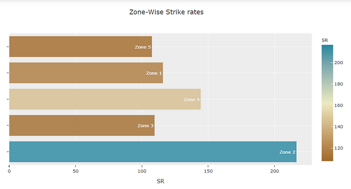
And After specific plotting, I have used barplots and Pie charts to analyze Strike rates, Runs scored, and dismissal for each of the 5 zones. Below is the screenshot of the same:


Interactive capabilities
The make this into an interactive web application I used Dash plotly. The key parameters which the user can select from are, Player and Last N matches.

For anyone wanting to learn Dash plotly and how to make these interactive web applications should follow Charming Data on youtube and study the documentation associated.
Lastly, deployed the web application on using Heroku: platform as a service (PaaS) that enables developers to build, run, and operate applications entirely in the cloud.
All the code related to the application can be found on my Github profile.
Conclusion
These plots can help you understand various aspects of a batter’s game, such as in which zone the batter is most vulnerable, the zone in which the batter has the highest strike rate and runs, implies that he/she might be the most comfortable handing deliveries in that particular zone.
All this information is invaluable when preparing for a match, we can have different plans for different batters to make the most of the vulnerabilities they possess in their style of playing.
Web Application : https://battingstrikingzones.herokuapp.com/